Forecasting the Israeli Elections using pymc3
Welcome!
For the political analysis of the final forecast, go here.
This post is a very technical discussion explaining how to run the model and reproduce the results of the final forecast.
Election polls are possibly the clearest and most public example of statistics that we encounter in our lives. We depend on them, as voters (or candidates), to understand where the election stands. They can contribute to tactical voting on the voters’ part, and can influence decisions on the part of candidates and politicians. But what do they mean? How does the margin-of-error figure into the numbers? What are we to understand if two polls have conflicting results? Here in Israel, the issue is even more pronounced: It is 2019, and there are currently over a dozen parties that have some viable chance of receiving some seats in parliament (called the Knesset). But a whole bunch of them are trailing near the “threshold.” The threshold - at 3.25% - means that if a party does not pass the threshold, its votes are divided up amongst the other parties using a complex algorithm called Bader-Ofer. Multiple polls taken at the same time might show different parties passing the threshold, and this naturally affects the final results.
This is the purpose of pyHoshen. pyHoshen is a framework for Bayesian MCMC election-polling written in pymc3. pymc3 is designed as an “Inference button” - just write the statistical model in high-level python and push the “Inference buttom” and it translates the code into a Bayesian MCMC model. Computing the model might take some time, but pymc3 uses C++ and the GPU to provide extra computational speed. Similarly, pyHoshen attempts to be the “Inference button” for election-polling - just feed in the polls and set up the election parameters, and it translates the polls into the statistical model for pymc3. This is a work-in-progress and contributions and comments are welcome!
It is important to understand - the model is a complex “poll of polls.” Whereas other poll of polls might provide a simple average, pyHoshen can account for correlations between parties and potential house effects of pollsters.
-
Correlations imply that the model might discern that two parties are negatively correlated. For example, they might be competing on the same electorate - if one party goes up, the corresponding party goes down and vice versa. This means that the results of the model will consider the correlations between the parties. If in a particular scenario that the model considers, the first party receives a higher support, the second will receive a lower support due to the correlations.
-
Normal polling error - Polls have an inherent error associated with them. The model accounts for this error by using a multivariate Student-T test for the polls.
-
House effects are the systematic tendencies of pollsters to give a better or worse percentage to a particular party beyond the normal polling error. We do not know if they are right or wrong in this, but we can determine that they systematically rank a party better or worse than the average. We use this to cancel out the “house effects” and determine where the average support for each party lies.
However, the model does not contain more information than the polls themselves. It is still just an elaborate poll of polls. If all the polls are wrong, or if the polls are on average wrong or off by some percentage points, the model will be wrong too.
Setup
So how do we run it? The following code was run on Google Colab, a free cloud computational environment. We start with the following initialization block which clones the pyHoshen repository and sets up the environment. I also authenticate to google for google docs, in order to access the polls database which is hosted at google sheets. Finally, we check the uptime. Google Colab only allows 12 hours of use at a time, and running the model can take over an hour or more. So if the uptime is close to the limit, it might be a good idea to reset the runtimes.
!rm -rf pyhoshen
!git clone https://github.com/byblian/pyhoshen.git

!rm -rf data
!git clone https://github.com/byblian/israel_election_data.git data

from google.colab import auth
auth.authenticate_user()

# setup hebrew-compatible fonts
!pip install python-bidi
import matplotlib
matplotlib.rc('font', family='DejaVu Sans')
!echo "-----------------------------------"
!echo -n "pyhoshen commit: " & GIT_DIR=`pwd`/pyhoshen/.git git rev-parse HEAD
!echo -n "data commit: " & GIT_DIR=`pwd`/data/.git git rev-parse HEAD

!date
!uptime
Cloning into 'pyhoshen'...
remote: Enumerating objects: 82, done.[K
remote: Counting objects: 100% (82/82), done.[K
remote: Compressing objects: 100% (55/55), done.[K
remote: Total 278 (delta 45), reused 60 (delta 25), pack-reused 196[K
Receiving objects: 100% (278/278), 1.49 MiB | 21.22 MiB/s, done.
Resolving deltas: 100% (143/143), done.
Cloning into 'data'...
remote: Enumerating objects: 38, done.[K
remote: Counting objects: 100% (38/38), done.[K
remote: Compressing objects: 100% (28/28), done.[K
remote: Total 38 (delta 17), reused 24 (delta 8), pack-reused 0[K
Unpacking objects: 100% (38/38), done.
Collecting python-bidi
Downloading https://files.pythonhosted.org/packages/e0/a7/ea6334b798546ed8584cb8cdc5d153c289294287b4ab46e9a4242480eae3/python_bidi-0.4.0-py2.py3-none-any.whl
Requirement already satisfied: six in /usr/local/lib/python3.6/dist-packages (from python-bidi) (1.11.0)
Installing collected packages: python-bidi
Successfully installed python-bidi-0.4.0
-----------------------------------
pyhoshen commit: 3aef2e5269590f4aa296a1ef3c31d338fc822462
data commit: c88cda97f2b3decc9c39b6c88812118c9c7a3746
Sun Apr 7 15:04:17 UTC 2019
15:04:19 up 1 min, 0 users, load average: 0.41, 0.20, 0.08
Having initialized let’s set up the model. Let’s go through the initialization parameters:
- forecast_day - We choose to forecast for election day
- house_effects_model - We use the “add-mean” model to account for house effects. This model specifies that each pollster has a certain additive factor for each party that is added to the actual party’s support at that time. There are various house effects models, but this seems to be the most stable and allows the model to converge.
- min_polls_per_pollster - To avoid throwing off the additive mean, we filter out pollsters that have only one poll. In practice, this meant we filtered out only one pollster.
- polls_since - We use all the polls since Feb 21, 2019 (the day the party lists were finalized)
- adjacent_day_fn - This function defines the prediction of a poll on adjacent days. In this case, we use \(e^{-diff}\), where diff is the offset in days.
- eta - A technical parameter that specifies the prior for the eta of the LKJ correlation matrix distribution.
import theano
theano.config.gcc.cxxflags = '-O3 -ffast-math -ftree-loop-distribution -funroll-loops -ftracer'
theano.config.allow_gc = False
theano.config.compute_test_value = 'off'

import numpy as np
import datetime
import pymc3 as pm
from pyhoshen import israel
forecast_day = None #datetime.date.today()
polls_since = datetime.datetime.strptime('21/02/2019', '%d/%m/%Y').date()
with pm.Model() as model:
  election = israel.IsraeliElectionForecastModel('data/elections.json',
      house_effects_model='add-mean', base_elections=[], eta=25,
      min_poll_days=35, polls_since=polls_since, forecast_day=forecast_day,
      min_polls_per_pollster=2, adjacent_day_fn=lambda diff: np.exp(-diff),
      forecast_election='election21_2019')
Some polls were filtered out. Provided polls: 59, filtered: 1, final total: 58
Running the model
All good, so let’s run it! The particular technical options below are useful to deal with some diagnostic warnings. In particular, “cores=2” forces google to run the two chains concurrently. Google Colab only has one CPU so pymc3 would normally run two chains sequentially by default. However, in my experience, “cores=2” runs faster (and possibly less buggy). In total, we will run 9,000 random scenarios or “draws” - 4500 on each of the two chains running concurrently. The first 2000 draws of each chain are used for tuning and discarded. They allow each chain to reach convergence to the final result. The final 2500 samples from each chain are going to constitute our final results, for a total of 5000 samples. Each of this sample is a unique possible way the election campaign could have unfolded to provide us the polls we see.
!uptime
with model:
  print (theano.config.gcc.cxxflags)
  print (election.forecast_election)
  print (election.forecast_model.house_effects_model)
  print ("forecast_day", election.forecast_model.forecast_day)
  nuts_kwargs=dict(target_accept=.8, max_treedepth=25, integrator='three-stage')
  samples = pm.sample(2500, tune=2000, cores=2, nutws_kwargs=nuts_kwargs)
 15:05:48 up 3 min,  0 users,  load average: 0.79, 0.39, 0.16


Auto-assigning NUTS sampler...
Initializing NUTS using jitter+adapt_diag...


-O3 -ffast-math -ftree-loop-distribution -funroll-loops -ftracer
election21_2019
add-mean
forecast_day 2019-04-09


WARNING (theano.tensor.blas): We did not find a dynamic library in the library_dir of the library we use for blas. If you use ATLAS, make sure to compile it with dynamics library.
Multiprocess sampling (2 chains in 2 jobs)
NUTS: [election21_2019_polls_pollster_house_effects, election21_2019_polls_innovations, election21_2019_votes, election21_2019_cholesky_pmatrix]
Sampling 2 chains: 100%|██████████| 9000/9000 [2:33:40<00:00,  1.19draws/s]
The model took us about 2.5 hours to complete! pymc3 will usually perform some diagnostics and warn us of them, if the model did not converge properly, for example. These warnings can imply errors or shortcomings in the model itself. But there are no warnings, meaning the model converged properly.
Analyzing and Visualizing the Results
The results we sampled only contain percentages of the various parties. As mentioned above, the Israeli parliament (Knesset) assigns seats based on an algorithm called Bader-Ofer, and election-polls are published using these Knesset seats. To convert the percentages we received to seats, we now compute the Bader-Ofer seat allocation for the entire trace. The trace is the set of all samples we got. Each of these samples contain a separate state of elections on each day of the election up to the forecast day. So we now run the Bader-Ofer algorithm separately on each of the days of each of the 5000 samples. We do it now because this is a heavy computation that is not necessary during the main run and would just slow down the computations. The model is a statistical model and uses a multivariate Student-T distribution to model the polls, and this requires percentages, not parliament seats.
import theano
theano.config.compute_test_value = 'off'
support_samples = samples['support']
bo=election.compute_trace_bader_ofer(support_samples)
Mandates Graph
So now we have the results! What can we see? The most standard display of poll results in Israel is the mandates bar graph. So we can just plot these.
election.plot_mandates(bo, hebrew=False)
election.plot_mandates(bo, hebrew=True)
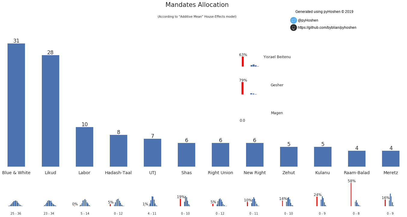
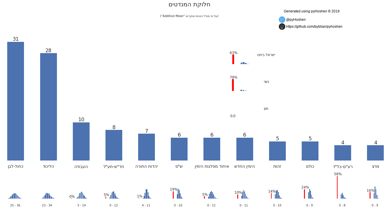
However, in addition to the normal bar graph that we are used to, we also see the distribution of each party’s support. We can see, for example, that “Kulanu” has a 76% of passing the threshold. Zehut - a type of libertarian 420-friendly party that is surprisingly making headway in the polls has an 86% chance of passing the threshold. Similarly, Raam-Balad, a union of two Arab parties that was almost blocked from running has a 58% chance of not passing the threshold.
Showing the distribution graphs for each party is nice but we also want to provide one final result. After the actual election, we might compare this final results to the true election election by determining the “error” it has – how far it is from the real true election results. A “Don’t be right, be smart!” approach is employed and the result that is presented is the one that has the lowest average “error” as compared to all other potential results.
Coalitions
Israeli elections are based on the formation of coalitions. To this end, we have coalition graphs, to see which potential coalitions are viable.
election.plot_coalitions(bo, hebrew=False)
election.plot_coalitions(bo, hebrew=True)
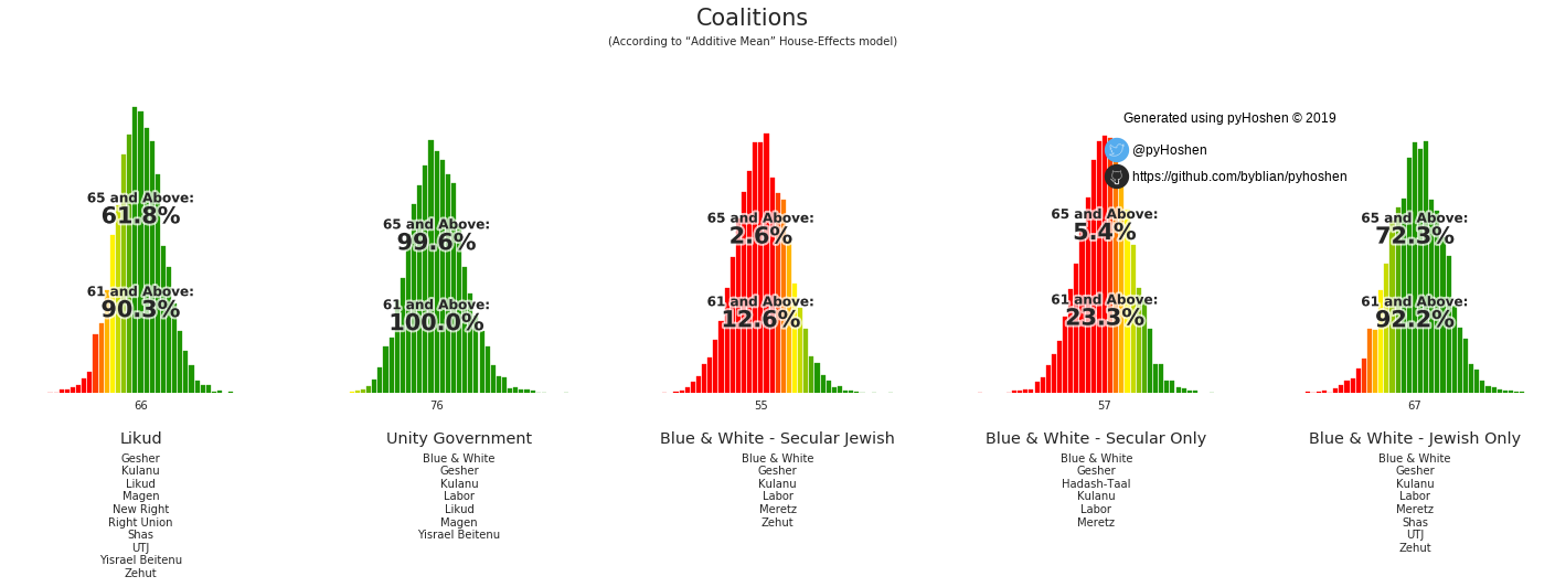
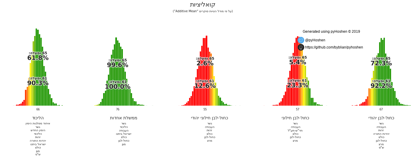
Based on the results above, it appears that the Likud has a good chance of forming a right-wing coalition. Furthermore, the average coalition size is 66 - suggesting that small parties that get 4 or 5 mandates would have less bargaining power during the coalition negotiations.
Party Support over Time
But our model did not just compute the final results, it also computed the results over time. We can plot these as well.
election.plot_party_support_evolution_graphs(support_samples, bo, hebrew=False)
election.plot_party_support_evolution_graphs(support_samples, bo, hebrew=True)
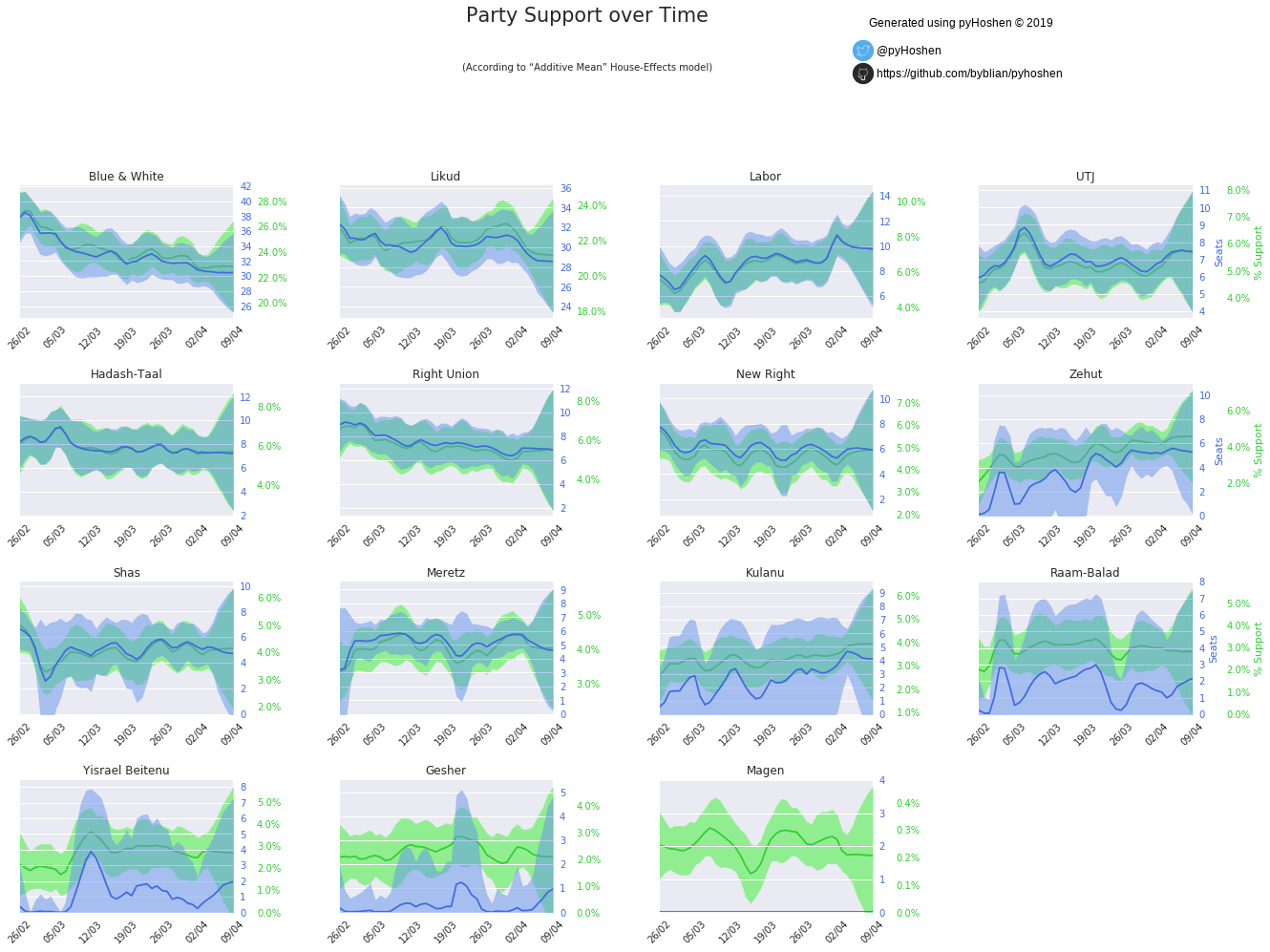
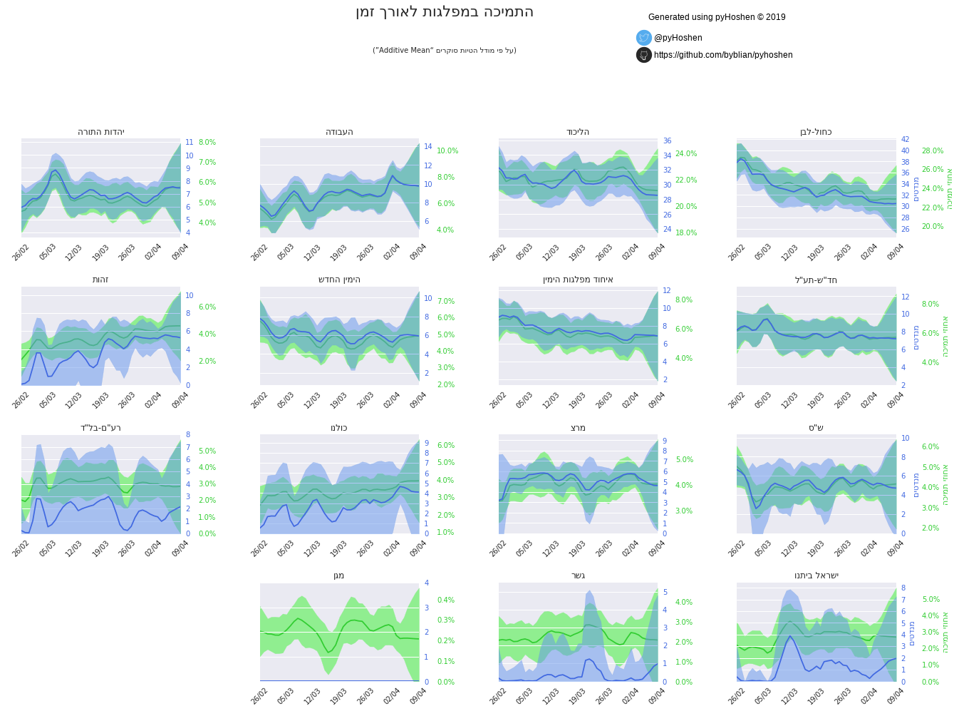
Most striking in the above graphs are the great uncertainty that develops over the last few days. In terms of a long-term outlook, we can see that Labor slowly rises as Blue & White slows decreases in power.
Technical sample details
As an initial first step to understand the diagnostics of sample, I run the following. The summary is a table of statistics for each random variable in the model. For example, each party’s percentage on each day is a separate random variable. Primarily, I look at the number of effective samples (n_eff) and Rhat. Rhat is the Gelman-Rubin statistic used to compare the results of the chains and should converge to 1 if the model converge. The n_eff indicates the the random variable with the lowest amount of effective samples has 2451 different effective samples, while the average effective samples in a variable is 6490. Similarly, we can see that the Gelman-Rubin statistic (Rhat) is 0.9998 at the lowest, 0.999939 on average, and 1.001832 at the maximum, all of which indicate good convergence.
import pymc3 as pm
summary = pm.summary(samples)
print ("min", summary.min())
print ("max", summary.max())
print ("mean", summary.mean())
min mean          -0.029975
sd             0.000000
mc_error       0.000000
hpd_2.5       -0.062274
hpd_97.5      -0.014019
n_eff       2451.686542
Rhat           0.999800
dtype: float64
max mean           1.000000
sd             0.023092
mc_error       0.000321
hpd_2.5        1.000000
hpd_97.5       1.000000
n_eff       9285.094114
Rhat           1.001832
dtype: float64
mean mean           0.062576
sd             0.006112
mc_error       0.000077
hpd_2.5        0.050626
hpd_97.5       0.074558
n_eff       6490.293947
Rhat           0.999939
dtype: float64
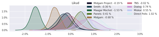
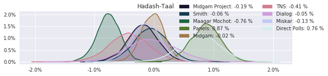
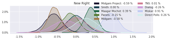
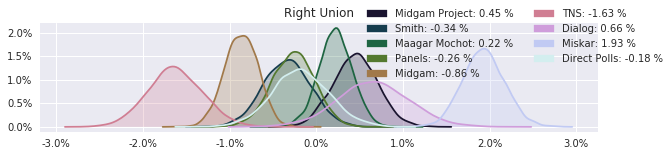
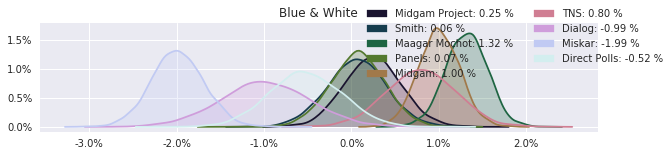
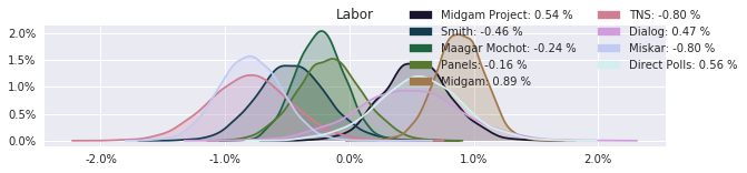
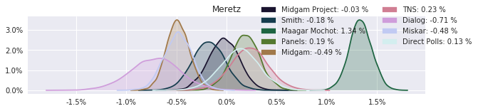
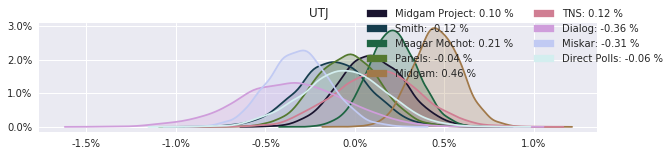
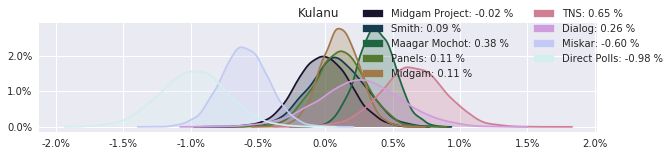
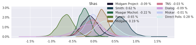
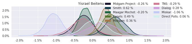
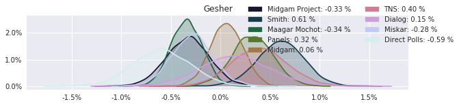
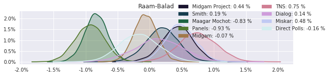
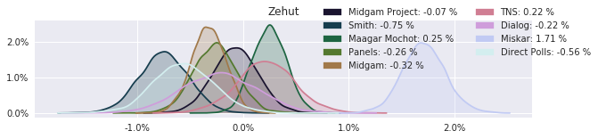
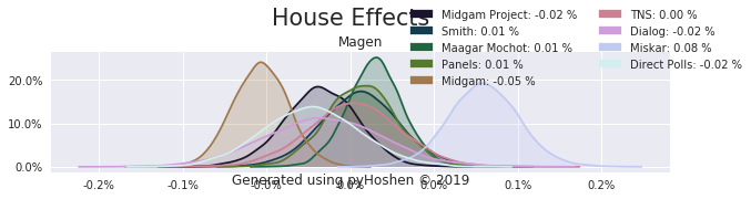
House Effects
The model also computed house effects so we can display these. We can see, for example, that “New Right” has a 0.26% extra house effect in “Direct Polls,” who is also that party’s private pollster. This translates to approximately a third of a mandate (1/120 = 0.83%). Similarly, a pollster called Miskar that published results only twice (and of these only once with full information), gave Zehut 7 mandates when everyone else gave it none. We see their house effect for Zehut is 1.71% - indicating heavy bias in favor of Zehut.
election.plot_pollster_house_effects(samples['election21_2019_polls_pollster_house_effects_b'], hebrew=False)
/usr/local/lib/python3.6/dist-packages/matplotlib/legend.py:508: UserWarning: Automatic legend placement (loc="best") not implemented for figure legend. Falling back on "upper right".
  warnings.warn('Automatic legend placement (loc="best") not '
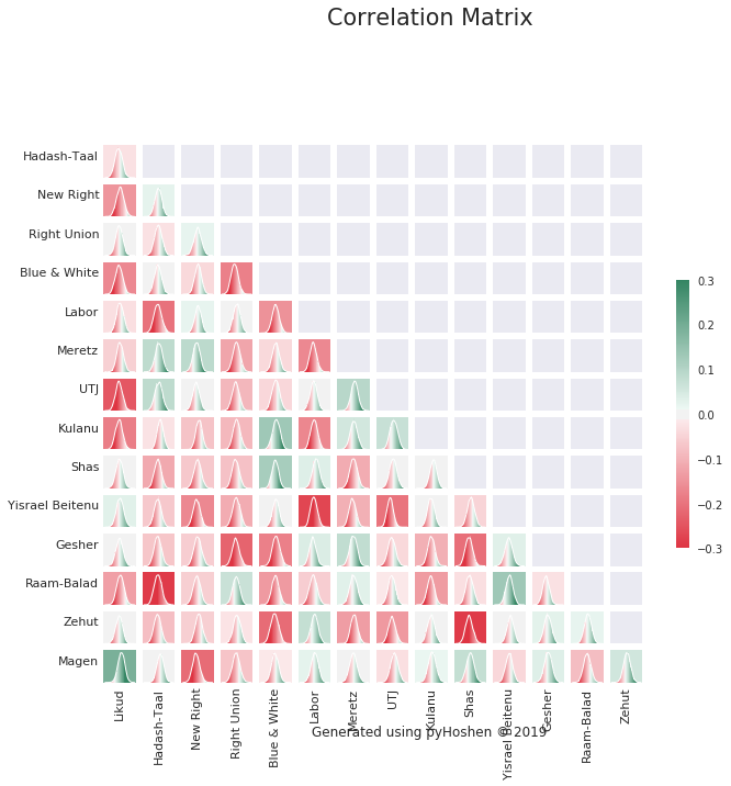
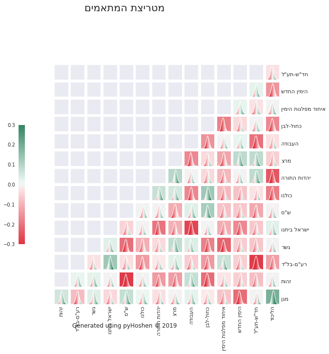
Correlation Matrix
Finally, we can plot our correlation distributions. Some of these make sense, while others do not. The model tries to make the best of what it can determine from the polls. With over a dozen parties competing, the model might make some false associations due to parties going up or down in polls the same day. It is a best effort, but in my opinion, better than simply assuming the respective party supports are totally unrelated. As an example, we can see the model was able to find heavy negative correlation between the two primary Arab parties - Hadash-Taal and Raam-Balad. This can be explained in terms of a common voter base, where their voters might choose one or the other. This in turn is taken into account when computing the final results. Thus, in the final mandate results, we might find either Hadash-Taal doing or Raam-Balad doing better. But the model would not simply randomly provide increased support for one or the other. It would come at the expense of the other.
from pyhoshen import utils
correlation_matrices = utils.compute_correlations(samples['election21_2019_cholesky_matrix'])
election.plot_election_correlation_matrices(correlation_matrices, hebrew=False)
election.plot_election_correlation_matrices(correlation_matrices, hebrew=True)